Data Cleaning
데이터 정리(Data Cleaning)는 데이터 과학의 핵심 부분입니다. 일부 텍스트 필드가 왜곡 되는 이유는 뭘까요? 결측값은 어떻게 해야할까요? 날짜 형식이 올바르지 않은 이유는 뭘까요? 일치하지 않는 데이터 입력을 어떻게 신속하게 정리할 수 있을까요? 이 과정에서는 이러한 문제가 발생하는 이유들과 해결하는 방법을 배워봅시다!
목차
- Handling Missing Values
- Scaling and Normalization
- Parsing Dates
- Character Encodings
- Inconsistent Data Entry
Handling Missing Values
데모를 위해 미식 축구 경기에서 발생한 이벤트 데이터 세트를 사용합니다.
1
2
3
4
5
6
7
8
9
# modules we'll use
import pandas as pd
import numpy as np

# read in all our data
nfl_data = pd.read_csv("input_data/NFL Play by Play 2009-2017 (v4).csv")

# set seed for reproducibility
np.random.seed(0)
데이터를 로드했으면 먼저, 일부 데이터를 출력하여 결측값이 있는지 확인해봅니다.
1
2
3
# look at the first five rows of the nfl_data file.
# I can see a handful of missing data already!
nfl_data.head()
1
2
3
4
5
6
7
8
9
10
11
12
13
14
15
16
17
18
19
20
21
22
         Date      GameID  Drive  qtr  down   time  TimeUnder  TimeSecs  \
0  2009-09-10  2009091000      1    1   NaN  15:00         15    3600.0
1  2009-09-10  2009091000      1    1   1.0  14:53         15    3593.0
2  2009-09-10  2009091000      1    1   2.0  14:16         15    3556.0
3  2009-09-10  2009091000      1    1   3.0  13:35         14    3515.0
4  2009-09-10  2009091000      1    1   4.0  13:27         14    3507.0

   PlayTimeDiff SideofField  ...    yacEPA  Home_WP_pre  Away_WP_pre  \
0           0.0         TEN  ...       NaN     0.485675     0.514325
1           7.0         PIT  ...  1.146076     0.546433     0.453567
2          37.0         PIT  ...       NaN     0.551088     0.448912
3          41.0         PIT  ... -5.031425     0.510793     0.489207
4           8.0         PIT  ...       NaN     0.461217     0.538783

   Home_WP_post  Away_WP_post  Win_Prob       WPA    airWPA    yacWPA  Season
0      0.546433      0.453567  0.485675  0.060758       NaN       NaN    2009
1      0.551088      0.448912  0.546433  0.004655 -0.032244  0.036899    2009
2      0.510793      0.489207  0.551088 -0.040295       NaN       NaN    2009
3      0.461217      0.538783  0.510793 -0.049576  0.106663 -0.156239    2009
4      0.558929      0.441071  0.461217  0.097712       NaN       NaN    2009

[5 rows x 102 columns]
결측값(NaN)이 몇 개 보입니다.
결측값을 얼마나 가지고 있을까요?
이제 우리는 결측값이 있다는 것을 압니다. 각 열에 몇 개가 있는지 보겠습니다.
1
2
3
4
5
# get the number of missing data points per column
missing_values_count = nfl_data.isnull().sum()

# look at the # of missing points in the first ten columns
missing_values_count[0:10]
1
2
3
4
5
6
7
8
9
10
11
Date                0
GameID              0
Drive               0
qtr                 0
down            61154
time              224
TimeUnder           0
TimeSecs          224
PlayTimeDiff      444
SideofField       528
dtype: int64
많은 것 같습니다! 이 문제의 규모를 더 잘 이해할 수 있도록 데이터 세트에서 결측값의 비율을 확인하는 것이 도움이 될 수 있습니다.
1
2
3
4
5
6
7
# how many total missing values do we have?
total_cells = np.product(nfl_data.shape)
total_missing = missing_values_count.sum()

# percent of data that is missing
percent_missing = (total_missing/total_cells) * 100
print(percent_missing)
1
24.87214126835169
이 데이터 세트에 있는 셀의 거의 1/4이 비어 있습니다! 다음 단계에서는 결측값이 있는 열 중 일부를 자세히 살펴보고 어떤 일이 벌어질지 알아내려고합니다.
결측값 데이터가 생기는 이유 파악하기
결측값이 생기는 이유를 파악하려면 직관적으로 데이터를 바라볼 필요가 있습니다. ‘이 값이 기록되지 않은 건지, 아니면 존재하지 않기 때문에 누락 된 것인지?’를 생각해봐야합니다. 예를 들어, ‘자녀가 없는 사람의 가장 큰 자녀의 키’ 데이터는 자녀가 없을 경우 값이 존재하지 않기 때문에 결측값이 됩니다. 이런 경우에는 데이터를 NaN으로 유지해야합니다. 반면에, 단순히 기록되지 않아서 결측값이 된 경우에는 해당 열과 행의 다른 값을 기반으로 추측하는 대치를 활용해야할 것입니다.
예를 들어 보겠습니다. nfl_data 데이터 프레임에서 결측값의 수를 보면 “TimesSec” 열에 많은 결측값이 있음을 알 수 있습니다.
1
2
# look at the # of missing points in the first ten columns
missing_values_count[0:10]
1
2
3
4
5
6
7
8
9
10
11
Date                0
GameID              0
Drive               0
qtr                 0
down            61154
time              224
TimeUnder           0
TimeSecs          224
PlayTimeDiff      444
SideofField       528
dtype: int64
결측값 없애기
바쁘거나 결측값 데이터를 분석할 이유가 없을 경우 차라리 결측값이 포함된 행이나 열을 제거하는 것도 한 방법입니다. pandas는 이를 수행하는데 편리한 함수인 dropna()를 가지고 있습니다.
1
2
# remove all the rows that contain a missing value
nfl_data.dropna()
하지만 이를 그대로 수행할 경우 단 하나의 데이터도 얻지 못할 수도 있습니다. 모든 행에 하나 이상의 결측값이 있을 수도 있기 때문입니다. 따라서, 적절한 데이터 세트를 얻기 위해 axis와 같은 매개변수를 추가해줄 수 있습니다.
1
2
3
# remove all columns with at least one missing value
columns_with_na_dropped = nfl_data.dropna(axis=1)
columns_with_na_dropped.head()
결측값을 제외하면 얼마나 많은 데이터를 잃게 되는지 확인해볼 필요가 있습니다.
1
2
3
# just how much data did we lose?
print("Columns in original dataset: %d \n" % nfl_data.shape[1])
print("Columns with na's dropped: %d" % columns_with_na_dropped.shape[1])
1
2
3
Columns in original dataset: 102

Columns with na's dropped: 41
결측값 대치하기
1
2
3
# get a small subset of the NFL dataset
subset_nfl_data = nfl_data.loc[:, 'EPA':'Season'].head()
subset_nfl_data
1
2
3
4
5
6
7
8
9
10
11
12
13
        EPA    airEPA    yacEPA  Home_WP_pre  Away_WP_pre  Home_WP_post  \
0  2.014474       NaN       NaN     0.485675     0.514325      0.546433
1  0.077907 -1.068169  1.146076     0.546433     0.453567      0.551088
2 -1.402760       NaN       NaN     0.551088     0.448912      0.510793
3 -1.712583  3.318841 -5.031425     0.510793     0.489207      0.461217
4  2.097796       NaN       NaN     0.461217     0.538783      0.558929

   Away_WP_post  Win_Prob       WPA    airWPA    yacWPA  Season
0      0.453567  0.485675  0.060758       NaN       NaN    2009
1      0.448912  0.546433  0.004655 -0.032244  0.036899    2009
2      0.489207  0.551088 -0.040295       NaN       NaN    2009
3      0.538783  0.510793 -0.049576  0.106663 -0.156239    2009
4      0.441071  0.461217  0.097712       NaN       NaN    2009
Panda의 fillna() 함수를 사용하여 데이터 프레임의 결측값을 채울 수 있습니다. 한 가지 옵션은 NaN 값을 대체 할 대상을 지정하는 것입니다. 여기서는 모든 NaN 값을 0으로 바꿉니다.
1
2
# replace all NA's with 0
subset_nfl_data.fillna(0)
1
2
3
4
5
6
7
8
9
10
11
12
13
        EPA    airEPA    yacEPA  Home_WP_pre  Away_WP_pre  Home_WP_post  \
0  2.014474  0.000000  0.000000     0.485675     0.514325      0.546433
1  0.077907 -1.068169  1.146076     0.546433     0.453567      0.551088
2 -1.402760  0.000000  0.000000     0.551088     0.448912      0.510793
3 -1.712583  3.318841 -5.031425     0.510793     0.489207      0.461217
4  2.097796  0.000000  0.000000     0.461217     0.538783      0.558929

   Away_WP_post  Win_Prob       WPA    airWPA    yacWPA  Season
0      0.453567  0.485675  0.060758  0.000000  0.000000    2009
1      0.448912  0.546433  0.004655 -0.032244  0.036899    2009
2      0.489207  0.551088 -0.040295  0.000000  0.000000    2009
3      0.538783  0.510793 -0.049576  0.106663 -0.156239    2009
4      0.441071  0.461217  0.097712  0.000000  0.000000    2009
결측값을 같은 열에서 바로 뒤에 오는 값으로 바꿀 수도 있습니다. (이것은 관측치에 일종의 논리적 순서가 있는 데이터 세트에서 의미를 가집니다.)
1
2
3
# replace all NA's the value that comes directly after it in the same column,
# then replace all the remaining na's with 0
subset_nfl_data.fillna(method='bfill', axis=0).fillna(0)
1
2
3
4
5
6
7
8
9
10
11
12
13
        EPA    airEPA    yacEPA  Home_WP_pre  Away_WP_pre  Home_WP_post  \
0  2.014474 -1.068169  1.146076     0.485675     0.514325      0.546433
1  0.077907 -1.068169  1.146076     0.546433     0.453567      0.551088
2 -1.402760  3.318841 -5.031425     0.551088     0.448912      0.510793
3 -1.712583  3.318841 -5.031425     0.510793     0.489207      0.461217
4  2.097796  0.000000  0.000000     0.461217     0.538783      0.558929

   Away_WP_post  Win_Prob       WPA    airWPA    yacWPA  Season
0      0.453567  0.485675  0.060758 -0.032244  0.036899    2009
1      0.448912  0.546433  0.004655 -0.032244  0.036899    2009
2      0.489207  0.551088 -0.040295  0.106663 -0.156239    2009
3      0.538783  0.510793 -0.049576  0.106663 -0.156239    2009
4      0.441071  0.461217  0.097712  0.000000  0.000000    2009
Scaling and Normalization
데이터를 스케일링하고 정규화하는 방법을 살펴봅시다.
1
2
3
4
5
6
7
8
9
10
11
12
13
14
15
16
# modules we'll use
import pandas as pd
import numpy as np

# for Box-Cox Transformation
from scipy import stats

# for min_max scaling
from mlxtend.preprocessing import minmax_scaling

# plotting modules
import seaborn as sns
import matplotlib.pyplot as plt

# set seed for reproducibility
np.random.seed(0)
Scaling vs. Normalization
스케일링과 정규화를 혼동하기 쉬운 이유 중 하나는 용어가 때때로 같은 의미로 사용되기 때문입니다. 두 경우 모두 변환 된 데이터 포인트가 유용한 특정 속성을 갖도록 숫자 변수의 값을 변환합니다. 차이점은 다음과 같습니다.
- 스케일링은 데이터 범위를 변경합니다.
- 정규화는 데이터 분포의 모양을 변경합니다.
Scaling
스케일링은 0-100 또는 0-1과 같이 특정 척도에 맞도록 데이터를 변환합니다. SVM(Support Vector Machine) 또는 KNN(k-nearest neighbors)과 같이 데이터 포인트가 얼마나 멀리 떨어져 있는지 측정하는 방법을 사용하는 경우 스케일링을 사용합니다. 이러한 알고리즘을 사용하면 숫자 피쳐의 “1”에 대한 변화가 동일한 중요도를 갖습니다.
일본 엔화와 미국 달러로 된 일부 제품의 가격을 예로 들어볼 수 있습니다. 1달러는 약 100엔의 가치가 있지만 스케일링 하지않으면 SVM 또는 KNN에서 1 엔의 가격 차이를 1 달러의 차이만큼 중요하게 간주합니다! 이것은 분명히 세상에 대한 상식에 맞지않습니다. 물론, 통화의 경우엔 환전하여 계산 할 수 있습니다. 하지만 키와 몸무게 같은 것을 예로 들면 어떨까요? 몇 kg이 몇 m와 같은지 명확하지 않습니다.
이런 상황에서 스케일링을 사용하면 다른 변수와 비교할 수 있게 됩니다.
1
2
3
4
5
6
7
8
9
10
11
12
# generate 1000 data points randomly drawn from an exponential distribution
original_data = np.random.exponential(size=1000)

# mix-max scale the data between 0 and 1
scaled_data = minmax_scaling(original_data, columns=[0])

# plot both together to compare
fig, ax = plt.subplots(1,2)
sns.distplot(original_data, ax=ax[0])
ax[0].set_title("Original Data")
sns.distplot(scaled_data, ax=ax[1])
ax[1].set_title("Scaled data")
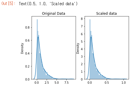
데이터의 모양은 변경되지 않았지만 0에서 8 범위가 0에서 1 사이로 스케일링 되었습니다.
Normalization
데이터 범위만 변경하는 스케일링과 다르게, 정규화는 관측치를 정규 분포로 설명 할 수 있도록 변경합니다.
일반적으로 데이터가 정규 분포를 따른다고 가정하는 기계 학습 또는 통계 기술을 사용하려는 경우 데이터를 정규화해야합니다. 이러한 예로는 선형 판별 분석(LDA) 및 Gaussian naive Bayes가 있습니다.(팁: 이름에 “Gaussian”이 포함 된 모든 방법은 아마도 정규화를 가정합니다.)
여기서 정규화하는 데 사용하는 방법을 Box-Cox 변환이라고합니다. 일부 데이터를 정규화하는 과정을 간단히 살펴 보겠습니다.
1
2
3
4
5
6
7
8
9
# normalize the exponential data with boxcox
normalized_data = stats.boxcox(original_data)

# plot both together to compare
fig, ax=plt.subplots(1,2)
sns.distplot(original_data, ax=ax[0])
ax[0].set_title("Original Data")
sns.distplot(normalized_data[0], ax=ax[1])
ax[1].set_title("Normalized data")
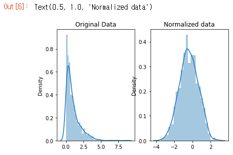
데이터의 모양이 변경되었습니다. 정규화하기 전에는 거의 L자 모양이었습니다. 그러나 정규화 후에는 종의 윤곽선(bell curve)처럼 보입니다.
Parsing Dates
2007년에서 2016년 사이에 발생한 산사태 데이터 세트를 사용해 작업해봅시다.
1
2
3
4
5
6
7
8
9
10
11
# modules we'll use
import pandas as pd
import numpy as np
import seaborn as sns
import datetime

# read in our data
landslides = pd.read_csv("input_data/catalog.csv")

# set seed for reproducibility
np.random.seed(0)
Check the data type of our date column
데이터의 처음 5개 행부터 살펴 보겠습니다.
1
landslides.head()
1
2
3
4
5
6
7
8
9
10
11
12
13
14
15
16
17
18
19
20
21
22
23
24
25
26
27
28
29
30
31
32
33
34
35
36
37
38
39
40
41
42
43
   id     date   time continent_code   country_name country_code  \
0  34   3/2/07  Night            NaN  United States           US
1  42  3/22/07    NaN            NaN  United States           US
2  56   4/6/07    NaN            NaN  United States           US
3  59  4/14/07    NaN            NaN         Canada           CA
4  61  4/15/07    NaN            NaN  United States           US

  state/province  population         city/town  distance  ...  \
0       Virginia       16000       Cherry Hill   3.40765  ...
1           Ohio       17288  New Philadelphia   3.33522  ...
2   Pennsylvania       15930       Wilkinsburg   2.91977  ...
3         Quebec       42786       Châteauguay   2.98682  ...
4       Kentucky        6903         Pikeville   5.66542  ...

                                 geolocation  hazard_type      landslide_type  \
0  (38.600900000000003, -77.268199999999993)    Landslide           Landslide
1  (40.517499999999998, -81.430499999999995)    Landslide           Landslide
2             (40.4377, -79.915999999999997)    Landslide           Landslide
3  (45.322600000000001, -73.777100000000004)    Landslide  Riverbank collapse
4  (37.432499999999997, -82.493099999999998)    Landslide           Landslide

  landslide_size   trigger storm_name injuries fatalities  \
0          Small      Rain        NaN      NaN        NaN
1          Small      Rain        NaN      NaN        NaN
2          Small      Rain        NaN      NaN        NaN
3          Small      Rain        NaN      NaN        NaN
4          Small  Downpour        NaN      NaN        0.0

                  source_name  \
0                  NBC 4 news
1              Canton Rep.com
2  The Pittsburgh Channel.com
3                   Le Soleil
4      Matthew Crawford (KGS)

                                         source_link
0      http://www.nbc4.com/news/11186871/detail.html
1  http://www.cantonrep.com/index.php?ID=345054&C...
2  https://web.archive.org/web/20080423132842/htt...
3  http://www.hebdos.net/lsc/edition162007/articl...
4                                                NaN

[5 rows x 23 columns]
landslides 데이터 프레임의 “date” 열로 작업 할 것입니다.
1
2
# print the first few rows of the date column
print(landslides['date'].head())
1
2
3
4
5
6
0     3/2/07
1    3/22/07
2     4/6/07
3    4/14/07
4    4/15/07
Name: date, dtype: object
데이터 유형이 object로 나옵니다. 인간인 우리가 보기엔 분명한 날짜형식이지만 파이썬은 이 데이터가 날짜 형식이라는걸 모릅니다. pandas dtype 문서를 보면 datatime64 dtype이 있습니다.
처음 몇 행을 인쇄하지 않아도 열의 dtype만 볼 수도 있습니다.
1
2
# check the data type of our date column
landslides['date'].dtype
1
dtype('O')
문자 코드를 dtype과 매칭하기 위해 numpy 문서를 확인해야할 수도 있습니다. ‘O’는 ‘object’의 문자 코드입니다.
Convert our date columns to datetime
이제 파이썬이 date 열을 날짜 형식으로 인식하도록 변환해봅시다. 문자열을 날짜 형식으로 변환하기 위해서 파이썬의 strftime을 참고합시다.
1
2
# create a new column, date_parsed, with the parsed dates
landslides['date_parsed'] = pd.to_datetime(landslides['date'], format="%m/%d/%y")
1
2
# print the first few rows
landslides['date_parsed'].head()
1
2
3
4
5
6
0   2007-03-02
1   2007-03-22
2   2007-04-06
3   2007-04-14
4   2007-04-15
Name: date_parsed, dtype: datetime64[ns]
날짜 데이터로 올바르게 파싱 되었습니다. 이제 유용하게 상호 작용할 수 있습니다!
- 여러 날짜 형식에서 오류가 발생하면 어떻게합니까? 여기서 날짜 형식을 지정하는 동안 단일 열에 여러 날짜 형식이있는 경우 오류가 발생하는 경우가 있습니다. 그럴 경우 pandas가 올바른 날짜 형식이 무엇인지 추론하도록합니다. 다음과 같이 할 수 있습니다.
1
landslides['date_parsed'] = pd.to_datetime(landslides['Date'], infer_datetime_format=True)
- 그럼 왜 항상 infer_datetime_format = True를 쓰지않나요? pandas가 항상 시간 형식을 추측하지 않는 데에는 두 가지 큰 이유가 있습니다. 첫 번째는 Pandas가 항상 올바른 날짜 형식을 알아낼 수는 없다는 것입니다. 특히 누군가가 데이터 입력을 창의적으로 사용한 경우에는 더욱 그렇습니다. 두 번째는 정확한 날짜 형식을 지정하는 것보다 훨씬 느리다는 것입니다.
Select the day of the month
이제 파싱 된 date 열이 있으므로 산사태가 발생한 날짜와 같은 정보를 추출 할 수 있습니다.
1
2
3
# get the day of the month from the date_parsed column
day_of_month_landslides = landslides['date_parsed'].dt.day
day_of_month_landslides.head()
1
2
3
4
5
6
0     2.0
1    22.0
2     6.0
3    14.0
4    15.0
Name: date_parsed, dtype: float64
Plot the day of the month to check the date parsing
날짜 데이터 파싱의 가장 큰 위험 중 하나는 월과 일을 섞는 것 입니다. to_datetime() 함수에는 매우 유용한 오류 메시지가 있지만 추출한 날짜가 의미있는 데이터인지는 다시 확인하는 것이 좋습니다.
이를 위해 해당 월의 날짜에 대한 히스토그램을 플로팅해봅시다. 우리는 1에서 31사이의 값을 가질 것이며, 산사태가 다른 날보다 더 흔하다고 생각할 이유가 없기 때문에 상대적으로 고른 분포를 보일 것이라 예상할 수 있습니다.
이것이 사실인지 살펴보겠습니다.
1
2
3
4
5
# remove na's
day_of_month_landslides = day_of_month_landslides.dropna()

# plot the day of the month
sns.distplot(day_of_month_landslides, kde=False, bins=31)
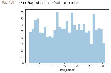
와우, 날짜 데이터를 올바르게 파싱한 것 같습니다! 이 그래프는 기대한 결과물입니다!
Character Encodings
먼저 필요한 라이브러리를 로드합시다!
1
2
3
4
5
6
7
8
9
# modules we'll use
import pandas as pd
import numpy as np

# helpful character encoding module
import chardet

# set seed for reproducibility
np.random.seed(0)
문자 인코딩이란?
문자 인코딩은 원시 이진 바이트 문자열(예: 0110100001101001)에서 사람이 읽을 수 있는 텍스트(예 : “hi”)를 구성하는 문자로 매핑하기위한 특정 규칙 집합입니다. 인코딩에는 여러 가지가 있으며 원래 작성된 것과 다른 인코딩으로 텍스트를 읽으려고하면 “모지 베이크”라는 스크램블 텍스트가 표시됩니다. 다음은 모지 베이크의 예입니다.
æ– ‡ å—化ã ??
“unknown” 문자로 끝날 수도 있습니다. 특정 바이트와 바이트 문자열을 읽는 데 사용하는 인코딩의 문자 사이에 매핑이 없을 때 인쇄되는 내용이 있으며 다음과 같습니다.
����������
문자 인코딩 불일치는 예전에 비해 많이 나아졌지만 여전히 문제가 됩니다. 다양한 문자 인코딩이 있지만 알아야 할 주요 인코딩은 UTF-8입니다.
UTF-8은 표준 텍스트 인코딩입니다. 모든 Python 코드는 UTF-8이며 이상적으로는 모든 데이터도 마찬가지입니다. 문제가 발생하는 것은 UTF-8이 아닐 때입니다.
Python2에서 인코딩을 처리하는 것은 꽤 어려웠지만 다행히 Python3에서는 훨씬 간단합니다. Python3에서 텍스트로 작업 할 때 접하게되는 두 가지 주요 데이터 유형이 있습니다. 하나는 기본적으로 텍스트인 문자열입니다.
1
2
3
4
5
# start with a string
before = "This is the euro symbol: €"

# check to see what datatype it is
type(before)
1
str
다른 하나는 정수 시퀀스인 bytes 데이터 유형입니다. 어떤 인코딩에 있는지 지정하여 문자열을 바이트로 변환 할 수 있습니다.
1
2
3
4
5
# encode it to a different encoding, replacing characters that raise errors
after = before.encode("utf-8", errors="replace")

# check the type
type(after)
1
bytes
bytes 객체를 보면 앞에 b가 있고 그 뒤에 텍스트가 있는 것을 볼 수 있습니다. 이는 바이트가 ASCII로 인코딩 된 문자인 것처럼 인쇄되기 때문입니다.(ASCII는 영어 이외의 다른 언어를 작성하는데 실제로 작동하지 않는 이전 문자 인코딩입니다.) 여기에서 유로 기호가 인쇄 될 때 ‘\xe2\x82\xac’와 같은 일부 모지 베이크로 대체되었음을 알 수 있습니다. 마치 ASCII 문자열 인 것처럼 말이죠.
1
2
# take a look at what the bytes look like
after
1
b'This is the euro symbol: \xe2\x82\xac'
바이트를 올바른 인코딩을 가진 문자열로 다시 디코딩하면 텍스트가 모두 올바르게 표기됨을 알 수 있습니다. :)
1
2
# convert it back to utf-8
print(after.decode("utf-8"))
1
This is the euro symbol: €
그러나 다른 인코딩을 사용하여 바이트를 문자열로 매핑하려고하면 오류가 발생합니다. 이는 우리가 사용하려는 인코딩이 전달하려는 바이트로 무엇을해야하는지 알지 못하기 때문입니다. 파이썬에게 바이트 문자열이 실제로 있어야하는 인코딩을 알려줘야합니다.
1
2
# try to decode our bytes with the ascii encoding
print(after.decode("ascii"))
1
2
3
4
5
6
7
---------------------------------------------------------------------------
UnicodeDecodeError                        Traceback (most recent call last)
<ipython-input-6-50fd8662e3ae> in <module>
      1 # try to decode our bytes with the ascii encoding
----> 2 print(after.decode("ascii"))

UnicodeDecodeError: 'ascii' codec can't decode byte 0xe2 in position 25: ordinal not in range(128)
잘못된 인코딩을 사용하여 문자열에서 바이트로 매핑하려고하면 문제가 발생할 수도 있습니다. 앞서 말했듯이, 문자열은 기본적으로 Python3에서 UTF-8이므로 다른 인코딩에있는 것처럼 처리하려고하면 문제가 발생합니다.
예를 들어, encode()를 사용하여 문자열을 ASCII용 바이트로 변환하려고하면 텍스트가 ASCII로되어있는 경우 바이트가 될 것을 요청할 수 있습니다. 하지만 텍스트가 ASCII가 아니기 때문에 처리 할 수 없는 문자가 있을 것입니다. ASCII가 처리 할 수 없는 문자를 자동으로 바꿀 수 있습니다. 그러나 그렇게하면 ASCII가 아닌 문자는 알 수 없는 문자로 대체됩니다. 그런 다음 바이트를 다시 문자열로 변환하면 해당 문자가 알 수 없는 문자로 대체됩니다. 이것에 대한 위험한 부분은 그것이 어떤 문자였어야 했는지 말할 방법이 없다는 것입니다. 즉, 데이터를 사용할 수 없게 만들었을 수도 있습니다!
1
2
3
4
5
6
7
8
9
10
11
# start with a string
before = "This is the euro symbol: €"

# encode it to a different encoding, replacing characters that raise errors
after = before.encode("ascii", errors = "replace")

# convert it back to utf-8
print(after.decode("ascii"))

# We've lost the original underlying byte string! It's been
# replaced with the underlying byte string for the unknown character :(
1
This is the euro symbol: ?
이것은 나쁘고 우리는 그것을 피하고 싶습니다! 가능한 한 빨리 모든 텍스트를 UTF-8로 변환하고 해당 인코딩으로 유지하는 것이 훨씬 좋습니다. UTF-8이 아닌 입력을 UTF-8로 변환하는 가장 좋은 시기는 파일을 읽을 때입니다. 다음에 대해 설명하겠습니다.
Reading in files with encoding problems
접하게 될 대부분의 파일은 아마도 UTF-8로 인코딩 될 것입니다. 이것이 파이썬이 기본적으로 기대하는 것이므로 대부분의 경우 문제가 발생하지 않습니다. 그러나 때때로 다음과 같은 오류가 발생합니다.
–> python3.9 & pandas 1.2.3 기준으로 인코딩 달라도 잘 열리는데(?)
만약 디코딩 에러가 발생할 경우 아래와 같이 해결합니다. 먼저, 어떤 인코딩이 사용되었는지 알아봅시다.
1
2
3
4
5
6
# look at the first ten thousand bytes to guess the character encoding
with open("input_data/ks-projects-201612.csv", 'rb') as rawdata:
    result = chardet.detect(rawdata.read(10000))

# check what the character encoding might be
print(result)
1
{'encoding': 'Windows-1254', 'confidence': 0.45794304475267217, 'language': 'Turkish'}
올바른 인코딩이 Windows-1254일 확률이 45%정도 됩니다.
1
2
3
4
5
# read in the file with the encoding detected by chardet
kickstarter_2016 = pd.read_csv("input_data/ks-projects-201612.csv", encoding='Windows-1252')

# look at the first few lines
kickstarter_2016.head()
–> 오히려 이렇게 할 경우 UnicodeDecodeError가 뜸…
UTF-8 인코딩으로 파일을 저장해줍니다.
1
2
# save our file (will be saved as UTF-8 by default!)
kickstarter_2016.to_csv("ks-projects-201801-utf8.csv")
Inconsistent Data Entry
먼저 라이브러리와 데이터를 로드해줍니다.
1
2
3
4
5
6
7
8
9
10
11
12
13
14
# modules we'll use
import pandas as pd
import numpy as np

# helpful modules
import fuzzywuzzy
from fuzzywuzzy import process
import chardet

# read in all our data
professors = pd.read_csv("input_data/pakistan_intellectual_capital.csv")

# set seed for reproducibility
np.random.seed(0)
Do some preliminary text pre-processing
1
professors.head()
1
2
3
4
5
6
7
8
9
10
11
12
13
14
15
16
17
18
19
20
21
22
23
24
25
26
27
28
29
30
31
32
33
34
   Unnamed: 0  S#         Teacher Name  \
0           2   3      Dr. Abdul Basit
1           4   5      Dr. Waheed Noor
2           5   6     Dr. Junaid Baber
3           6   7  Dr. Maheen Bakhtyar
4          24  25          Samina Azim

            University Currently Teaching             Department  \
0               University of Balochistan  Computer Science & IT
1               University of Balochistan  Computer Science & IT
2               University of Balochistan  Computer Science & IT
3               University of Balochistan  Computer Science & IT
4  Sardar Bahadur Khan Women's University       Computer Science

  Province University Located          Designation Terminal Degree  \
0                 Balochistan  Assistant Professor             PhD
1                 Balochistan  Assistant Professor             PhD
2                 Balochistan  Assistant Professor             PhD
3                 Balochistan  Assistant Professor             PhD
4                 Balochistan             Lecturer              BS

                                      Graduated from   Country    Year  \
0                      Asian Institute of Technology  Thailand     NaN
1                      Asian Institute of Technology  Thailand     NaN
2                      Asian Institute of Technology  Thailand     NaN
3                      Asian Institute of Technology  Thailand     NaN
4  Balochistan University of Information Technolo...  Pakistan  2005.0

           Area of Specialization/Research Interests Other Information
0                        Software Engineering & DBMS               NaN
1                                               DBMS               NaN
2          Information processing, Multimedia mining               NaN
3  NLP, Information Retrieval, Question Answering...               NaN
4                      VLSI Electronics DLD Database               NaN
데이터 입력 불일치가 없는지 확인하기 위해 “Country” 열을 정리하는데 관심이 있다고 가정해보겠습니다. 물론 각 행을 직접 살펴보고 직접 확인할 수 있으며 불일치를 발견하면 직접 수정할 수 있습니다. 하지만 더 효율적인 방법이 있습니다!
1
2
3
4
5
6
# get all the unique values in the 'Country' column
countries = professors['Country'].unique()

# sort them alphabetically and then take a closer look
countries.sort()
countries
1
2
3
4
5
6
7
8
array([' Germany', ' New Zealand', ' Sweden', ' USA', 'Australia',
       'Austria', 'Canada', 'China', 'Finland', 'France', 'Greece',
       'HongKong', 'Ireland', 'Italy', 'Japan', 'Macau', 'Malaysia',
       'Mauritius', 'Netherland', 'New Zealand', 'Norway', 'Pakistan',
       'Portugal', 'Russian Federation', 'Saudi Arabia', 'Scotland',
       'Singapore', 'South Korea', 'SouthKorea', 'Spain', 'Sweden',
       'Thailand', 'Turkey', 'UK', 'USA', 'USofA', 'Urbana', 'germany'],
      dtype=object)
이걸 보면 ‘ Germany’와 ‘germany’, ‘ New Zealand’와 ‘New Zealand’ 같은 데이터 입력이 일치하지 않아 문제가 있음을 알 수 있습니다.
가장 먼저 할 일은 모든 것을 소문자로 만들고 시작과 끝 부분의 공백을 제거하는 것입니다. 대소문자의 불일치 및 후행 공백은 텍스트 데이터에서 매우 일반적이며 이렇게하면 텍스트 데이터 입력 불일치의 80%를 수정할 수 있습니다.
1
2
3
4
# convert to lower case
professors['Country'] = professors['Country'].str.lower()
# remove trailing white spaces
professors['Country'] = professors['Country'].str.strip()
다음으로, 더 어려운 불일치를 해결해보겠습니다.
Use fuzzy matching to correct inconsistent data entry
‘Country’열을 다시 살펴보고 데이터 정리가 더 필요한지 확인하겠습니다.
1
2
3
4
5
6
# get all the unique values in the 'Country' column
countries = professors['Country'].unique()

# sort them alphabetically and then take a closer look
countries.sort()
countries
1
2
3
4
5
6
7
array(['australia', 'austria', 'canada', 'china', 'finland', 'france',
       'germany', 'greece', 'hongkong', 'ireland', 'italy', 'japan',
       'macau', 'malaysia', 'mauritius', 'netherland', 'new zealand',
       'norway', 'pakistan', 'portugal', 'russian federation',
       'saudi arabia', 'scotland', 'singapore', 'south korea',
       'southkorea', 'spain', 'sweden', 'thailand', 'turkey', 'uk',
       'urbana', 'usa', 'usofa'], dtype=object)
또 다른 불일치가 있는 것 같습니다. ‘southkorea’와 ‘south korea’는 동일해야합니다.
fuzzywuzzy 라이브러리를 사용하여 서로 가장 가까운 문자열을 식별 할 것 입니다. 이 데이터 세트는 손으로 오류를 수정할 수 있을만큼 작지만, 이런 접근 방식은 확장성이 좋지 않습니다. (수작업으로 수천 개의 오류를 수정 하시겠습니까? 1만 개 정도는 어떻습니까? 일반적으로 가능한 한 빨리 자동화하는 것이 좋습니다.)
Fuzzy matching: 대상 문자열과 매우 유사한 텍스트 문자열을 자동으로 찾는 프로세스입니다. 일반적으로 문자열은 다른 문자열에 “가까운” 것으로 간주되며 한 문자열을 다른 문자열로 변환하는 경우 변경해야하는 문자 수가 적습니다. 따라서 “apple”과 “snapple”은 “s”와 “n”을 추가하는 동시에 “in”과 “on”을 두 번 변경하고 “i”를 “o”로 바꿉니다. 퍼지 매칭에 항상 100 % 의존 할 수있는 것은 아니지만 일반적으로 최소한 시간을 절약 할 수 있습니다.
Fuzzywuzzy는 주어진 두 문자열의 비율을 반환합니다. 비율이 100에 가까울수록 두 문자열 사이의 편집 거리가 작아집니다. 여기서는 “d.i khan”과 가장 가까운 거리에있는 도시 목록에서 10개의 문자열을 가져옵니다.
1
2
3
4
5
# get the top 10 closest matches to "south korea"
matches = fuzzywuzzy.process.extract("south korea", countries, limit=10, scorer=fuzzywuzzy.fuzz.token_sort_ratio)

# take a look at them
matches
1
2
3
4
5
6
7
8
9
10
[('south korea', 100),
 ('southkorea', 48),
 ('saudi arabia', 43),
 ('norway', 35),
 ('ireland', 33),
 ('portugal', 32),
 ('singapore', 30),
 ('netherland', 29),
 ('macau', 25),
 ('usofa', 25)]
“south korea”와 “southkorea” 두 항목이 “south korea”에 매우 가깝다는 것을 알 수 있습니다. 비율이 47보다 큰 “Country” 열의 모든 행을 “south korea”으로 바꿉니다.
재사용성을 위해 함수로 작성하겠습니다.
1
2
3
4
5
6
7
8
9
10
11
12
13
14
15
16
17
18
19
20
21
22
23
24
# function to replace rows in the provided column of the provided dataframe
# that match the provided string above the provided ratio with the provided string
def replace_matches_in_column(df, column, string_to_match, min_ratio=47):
   # get a list of unique strings
   strings = df[column].unique()

   # get the top 10 closest matches to our input string
   matches = fuzzywuzzy.process.extract(
      string_to_match, strings,
      limit=10,
      scorer=fuzzywuzzy.fuzz.token_sort_ratio
   )

   # only get matches with a ratio > 90
   close_matches = [matches[0] for matches in matches if matches[1] >= min_ratio]

   # get the rows of all the close matches in our dataframe
   rows_with_matches = df[column].isin(close_matches)

   # replace all rows with close matches with the input matches
   df.loc[rows_with_matches, column] = string_to_match

   # let us know the function's done
   print("All done!")
이제 만든 함수를 사용해봅시다!
1
2
# use the function we just wrote to replace close matches to "south korea" with "south korea"
replace_matches_in_column(df=professors, column='Country', string_to_match="south korea")
1
All done!
이제 “Country”열의 고유값을 다시 확인하고 “south korea”를 올바르게 정리했는지 확인합니다.
1
2
3
4
5
6
# get all the unique values in the 'Country' column
countries = professors['Country'].unique()

# sort them alphabetically and then take a closer look
countries.sort()
countries
1
2
3
4
5
6
7
array(['australia', 'austria', 'canada', 'china', 'finland', 'france',
       'germany', 'greece', 'hongkong', 'ireland', 'italy', 'japan',
       'macau', 'malaysia', 'mauritius', 'netherland', 'new zealand',
       'norway', 'pakistan', 'portugal', 'russian federation',
       'saudi arabia', 'scotland', 'singapore', 'south korea', 'spain',
       'sweden', 'thailand', 'turkey', 'uk', 'urbana', 'usa', 'usofa'],
      dtype=object)
잘 정리되었습니다! :)